
TextDNA Instructions for Use
Data Format
TextDNA reads SQLite databases representing ordered sequences (genomes) of elements (genes) and optionally subsequences within the original sequences (chromosomes). For the purpose of comparison between elements of different sequences, matching sets of elements are identified by an integer label (the ortholog_group_id).
The basic schema for the database file is as follows (elements in italics are descriptions of the column data and NOT part of the schema):
|
TABLE genome |
||
|
genome_id |
integer PRIMARY KEY |
Default ordering of the sequences. Should start with zero and continue in counting order (i.e. 0, 1, 2, ...). |
| name | text | name of the sequence |
|
TABLE chromosome |
||
| chromosome_id | integer PRIMARY KEY | Numeric identifier for a subsequence. Should start with zero and continue in counting order (i.e. 0, 1, 2, ...). |
| name | text | name of the subsequence |
| genome_id | integer | genome_id of parent sequence |
| length | integer | number of elements in the subsequence |
|
TABLE gene |
||
| gene_id | integer PRIMARY KEY | Numeric identifier for an element. Should start with zero and continue in counting order (i.e. 0, 1, 2, ...). |
| name | text | name of the element |
| description | text | textual description of the element |
| chromosome_id | integer | chromosome_id of the parent subsequence |
| index_in_chromosome | integer | order of the element within the subsequence |
| start | integer | absolute starting position of the element within the subsequence |
| end | integer | absolute ending position of the element within the subsequence |
| strand | integer | 0 or 1 |
| ortholog_group_id | integer | Numeric identifier for a set of matching elements. Should start with zero and continue in counting order (i.e. 0, 1, 2, ...). |
The Google N-Grams data included with this software represents the 1,000 most popular words per decade from 1660 to 2000 according to Google (see http://books.google.com/ngrams/info for the original count data). In the case of the Google N-Grams data, column data is as follows:
TABLE genome |
Describes the properties of a decade | |
genome_id |
integer PRIMARY KEY |
Default ordering of the decades |
| name | text | Name of the decade (e.g. 1660) |
TABLE chromosome |
A second object for defining decades | |
| chromosome_id | integer PRIMARY KEY | Numeric identifier for the decade |
| name | text | Arbitrary name |
| genome_id | integer | Numeric identifier of the decade in the genome table |
| length | integer | The number of words in the decade (e.g. 1000) |
TABLE gene |
Describes information about an instance of a word | |
| gene_id | integer PRIMARY KEY | Numeric identifier for a word |
| name | text | The word itself |
| description | text | Additional information about the word from the Google database |
| chromosome_id | integer | The chromosome_id of the parent decade |
| index_in_chromosome | integer | The rank of of the popularity of the word within the parent decade |
| start | integer | The normalized inverse log of the number of instances of the word in the parent decade |
| end | integer | The normalized inverse log of the one more than number of instances of the word in the parent decade |
| strand | integer | 1 |
| ortholog_group_id | integer | A numeric identifier for all instances of the word (i.e. all instances of 'the' map to 1) |
Additional data about the elements can be added to the gene table by adding a new column. Any additional information must be of a numeric form (one of "int", "integer", "tinyint", "smallint", "mediumint", "bigint","unsigned big int", "int2", "int8", "real", "double", "double precision", "float", "numeric", "decimal(10,5)", "boolean") and can then be used as a mapping to color individual elements in the tool (see "Customizing the Display").
Data can also be added through CSV files. The files must be of the format:
<set_name>, <element_name>, <position_in_set>, <count_value>
where each entry is located on a separate line. The number of elements loaded can be set by setting an upper bound on the "rank" value (see "Customizing the Display"). All datasets must use matching element_name values to define matching element names.
Display Overview
|
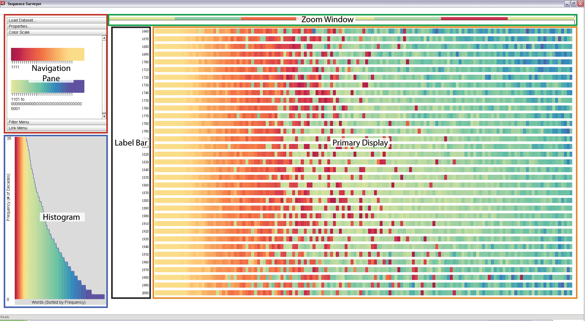
TextDNA leverages multiple visual displays to support visual analysis. The above image is the default TextDNA screen that appears when first loading a dataset. The components are as follows:
- Primary Display: An overview display of the data. Sequences map to rows; elements map to colors within the rows.
- Zoom Window: A detailed view of a specific blocked region within a row as selected by the user.
- Label Bar: The names of the sequences represented by each row. Names are aligned with the sequence rows that they represent.
- Histogram: A distribution of the matching sets of elements by frequency within the data (matching elements refer to elements with same ortholog_group_id field (see "Data Format" for details)). Elements are sorted along the x-axis according to the number of elements in the matching set and colored with respect to the color parameters of the primary display. The height of an element bar represents the average frequency of the element sets represented by the bar; the blue line traces the maximal matching set frequency represented by the bar.
- Navigation Pane: This panel contains a variety of options for interacting with and exploring the data in the primary display. The components of this pane will be described in more detail in the section on "Customizing the Display".
Interacting with different elements of the display can affect other display components. For more detailed information on interaction with the various componenets of the display, see the ensuing sections of this guide.
Basic Use
To load a dataset into TextDNA, select the "Load Dataset" tab from the Navigation Pane. Click on the "Load" button to open the load file dialog box and navigate to the desired dataset on your computer (NOTE: files must have .db, .sql, or .sqlite extensions). Select the file and click "Open" to load the data into the tool.
The default display orders sequence rows in the Primary Display by their genome_id field (see "Data Format" for details). Rows can be rearranged by holding down the Alt key and clicking and dragging sequence rows vertically within the display. The names of each sequence are displayed in the Label Bar beside their respective sequence rows. Within each row, neighboring elements are grouped into blocks, collections of data elements aggregated spatially according to the Block Width parameter (see "Customizing the Display" for details). By default, each block is displayed as the average color of genes within the region represented by the block; however, alternative visual representations of the blocks are available.
 |
Elements within a particular spatial region are grouped into a single glyph, called a block. The width and representation of a block can be controlled by the user. |
Mousing over a block in the Primary Display will reveal a tooltip containing the names of elements within the block, followed by the subsequence name and sequence name on a separate line. If there are a large number of elements within a block, the list of names may be truncated, as indicated by an ellipse. Mousing over a block will also highlight any blocks in the Primary Display containing at least one element matching an element in the current block, the locations of the elements in the Histogram display, and the corresponding elements in the Zoom Window, if locked. Clicking on a block in the Primary Display will cause lines to be drawn between all blocks containing at least one element matching an element in the clicked block. Links are only drawn between blocks sharing a matching element. Clicking on the block again will remove the lines. Right clicking on any block and selecting "Clear Links" will remove all lines from the Primary Display.
Detailed information about the contents of a block can be accessed through the Primary Display. Right clicking on a block and selecting "View Component Text" will display the names of elements within a block, separated by blank lines, in a pop-up window. Right clicking and selecting "Details" will open a pop-up containing a list of sequences in which elements matching the components of the clicked block can be found. Selecting a sequence name displays information about the matched element in that sequence, including information from the description field of the database. Elements are indicated by '*' and blocks are separated by '***'. The blocks from the genome initially selected are preceded by "Target:" in the genome window.
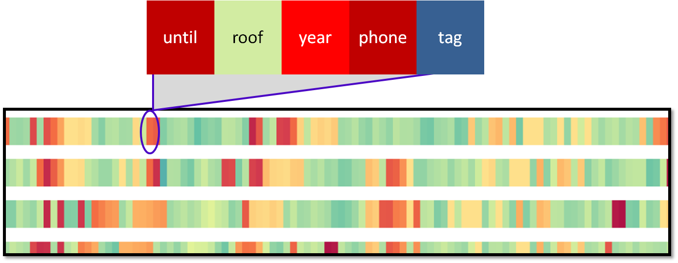
Elements contained within a block can also be explored in the Zoom Window. Mousing over a block in the Primary Display will cause the components of the block to be displayed in the Zoom Window. Elements are displayed on either side of a horizontal guide line on the basis of their strand field (see "Data Format" for details). The elements are represented as colored rectangles: their color and positioning correspond to their color and position values as defined by the parameters of the Primary Display. To interact with the components of the locked block, right click on the block in the primary display and select "Zoom to Block". The block is then locked into the Zoom Window and outlined in the Primary Display. If the component elements in the Zoom Window are dense, they may be aggregated into blocks, in which case, a zoomed block can be further explored by again locking the block in the Zoom Window.
Once locked, mousing over an element will highlight blocks in the Primary Display containing that element, sequences in the Label Bar where the element is found and the location of the element in the Histogram distribution. Clicking on a block will draw a connecting link between blocks containing that element in the primary display. Clicking again will remove the link. Right click on any block in the Primary Display or Zoom Window and select "Unlock Zoomed Block" to release the block from the Zoom Window and return to mouseover zoom in the Primary Display.
Mousing over a bar in the histogram display creates a tooltip with the list of ortholog_group_id values of the matched sets of elements represented by the bars. It highlights sequences containing those elements in the Label Bar and the corresponding blocks containing the elements in the Primary Display. Clicking and dragging the mouse in the Histogram display draws a red rectangle in the Histogram. Releasing the mouse filters the data in the primary view: blocks containing elements corresponding to the bars within the rectangle remain fully opaque, while all other blocks are made partially transparent. Pressing escape removes this filter and clears the Histogram display.
Customizing the Display
The Navigation Pane contains a variety of menus for customizing the display. Selecting a tab in the Navigation Pane will open the corresponding menu set. This section will discuss these menus and how they can be used to support analysis in TextDNA. See the paper for details and examples of the types of analysis that these customizations can support.
Load Dataset
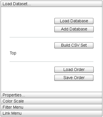 |
The "Load Dataset" menu contains options for interacting with and changing the underlying data of the display. |
- "Load" button: Opens a load file dialog box to load a new dataset into TextDNA. The new dataset will replace the currently visualized database. The dataset file name will appear to the left of the button.
- "Add Database" button: Opens a load file dialog box to add a new dataset to the existing TextDNA display. Matching sets between the new and existing datasets are created by matching element names between the two datasets. The dataset file name of the added database will appear to the left of the button.
- "Build CSV Set" button: Opens a window for customizing a CSV-based dataset. Selecting "Add File" opens a file load dialog box, where you can select a CSV display file. Selected files populate the top list window. Selecting files in the "CSV File" window and then selecting "Delete Selected" will remove the selected files from the dataset. Setting the "Top N" value sets the upper bound on element rank values displayed from the file. On opening a file, this bound will be set to the maximum rank from the file set. Click "OK" to build a new dataset from the listed files and "Top N" value or cancel to cancel the file build. Selecting the "Build CSV Set" button will allow you to make changes to the CSV dataset parameters on the fly.
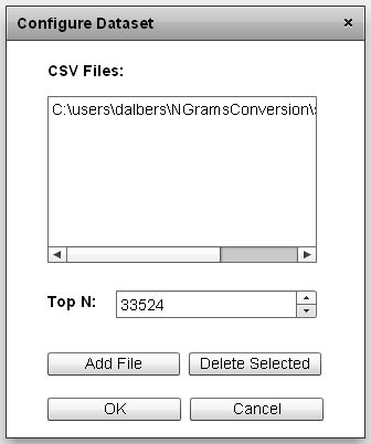 |
The CSV dataset configuration window. Files for the dataset are located in the upper window. The upper boundary on the rank value is set by the Top N value. |
- "Load Order" button: Opens a file load dialog box to locate a .csv file containing the names of the sequences in their desired order from top to bottom (e.g. top_sequence_name, second_sequence_name,..., bottom_sequence_name). If the sequence names do not match the active dataset, the default ordering will instead be used.
- "Save Order" button: Opens a file save dialog box to save a .csv file containing the current order of sequences in the display from top to bottom.
Properties
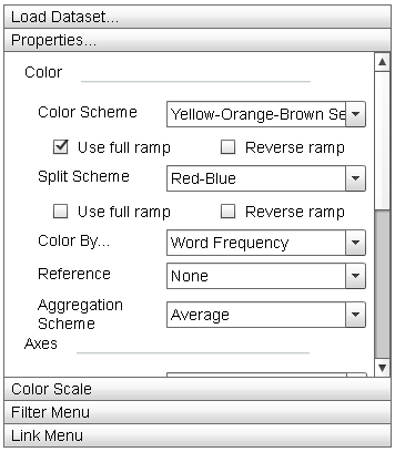 |
The "Properties" menu allows the user to manipulate the display parameters of the Primary Display. The "Update" button adjusts the parameters of the display to match those set in this menu. |
- "Color" Menu Section:
This menu section contains parameter settings for changing the element color mapping properties of the Primary Display, Zoom Window, and Histogram.
- "Color Scheme" dropdown list: This dropdown contains the actual color ramps that are mapped to elements. By default, TextDNA offers nine different color ramps and a grey ramp. Other colors can be added by clicking the "Add Custom Color" button. Selecting the "Reverse ramp" checkbox below the dropdown list will invert the ramp before applying it to the data. Selecting the "Use full ramp" checkbox will cause the entire ramp to be used when using split color encodings.
- "Secondary Scheme" dropdown list: This dropdown is used to specify the secondary color ramps used when using split color encodings. If the same ramp is specified in both the "Color Scheme" and "Secondary Scheme" lists, split encodings will use the first half of the ramp as the "Color Scheme" and the second half as the "Secondary Scheme".
- "Color By" dropdown list: This list defines the property of an element that is mapped to the element color. There are six default property colorings. Additional colorings may be added by adding additional columns to the input database (see "Data Format" for details). Valid supplemental colorings are referenced by column name in this list. "Grouped Frequency Ordering" and "Position in Reference" are split coloring properties: a portion of the elements are mapped to one ramp while the remainder are mapped to another.
- Grouped Frequency Ordering: Sets of matching elements are colored according to the set of sequences in which the elements are found. A total ordering is achieved by further sorting elements by their overall frequency (i.e. the number of matching elements in the set), their position in the sequences in decending order, and their ortholog_group_id value respectively. Matching element sets with at least one element in each sequence are mapped to the "Color Scheme" ramp, while the remaining are mapped to the "Secondary Scheme" ramp. This property highlights patterns of co-occurence between matching sets of elements: in the context of the N-Grams data, words appearing among the top 1,000 most popular in the same series of decades will be colored similarly.
- Membership Frequency: Sets of matching elements are colored according to the number of sequences they appear in. For instance, in the context of the N-Grams data, words appearing among the top 1,000 most popular in the same number of decades will be colored identically.
- Number of Matches: Elements are colored according to their start value (see "Data Format" for details). In the context of the N-Grams data, this value is the normalized inverse log of the number of instances a particular word was found in the Google Books database for that particular decade. (NOTE: Since this value is variable per set of matching elements, the Histogram is colored using a constant value.)
- Position in Reference: Elements are colored according to the position of the first matching element in a target sequence. This sequence can either be selected through the "Reference" dropdown list immediately below the "Color By" dropdown list or by right clicking on a target seqeunce and selecting "Set as Color Reference". Elements matching elements in the reference are colored according to the "Color Scheme" ramp and remaining elements are colored according to the "Secondary Scheme" ramp, with colors being assigned according to the order in which a matching element is first found in the remaining sequences, from top to bottom. This coloring highlights the movement of elements from one sequence across the remaining sequences.
- Word Frequency: An element is colored according to the number of elements matching it within the dataset. This differs from membership frequency as it considers elements occuring multiple times within a single decade separately.
- Word Index: Elements are colored according to their relative position within a sequence. For example, in the N-Grams data, words would be colored according to their popularity within a decade. This coloring can be used to highlight positional patterns between sequences. (NOTE: Since this value is variable per set of matching elements, the Histogram is colored using a constant value.)
- "Aggregation Scheme" dropdown list: TextDNA offers four block encodings which display different statistical properties of the colors of the elements represented by the block.
- Average: Each block is represented as a solid color representing the average value of the "Color By" parameter across elements in the block.
- Color Weaving: Each block represents the approximate distribution of values of the "Color By" parameters across elements in the block. Each pixel is mapped to the value of one element. After each element is mapped to a pixel, the elements are randomized and mapped to the remaining pixels. The randomization repeats until the block is filled.
- Event Striping: This aggregation method highlights outliers and points of change within a block. Outliers (a data value greater than 1.5 times the inner quartile mean of values in the block) are mapped as stripes on the block. Dominant changes to the average value are visible as immediate shifts in the background color.
- Robust Average: Each block is represented as a solid color representing the average value of the "Color By" parameter across the elements in the block, excluding local outlier values.
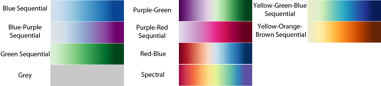
TextDNA supports nine Color Brewer color schemes and a solid grey scheme. User-defined ramps are also supported.
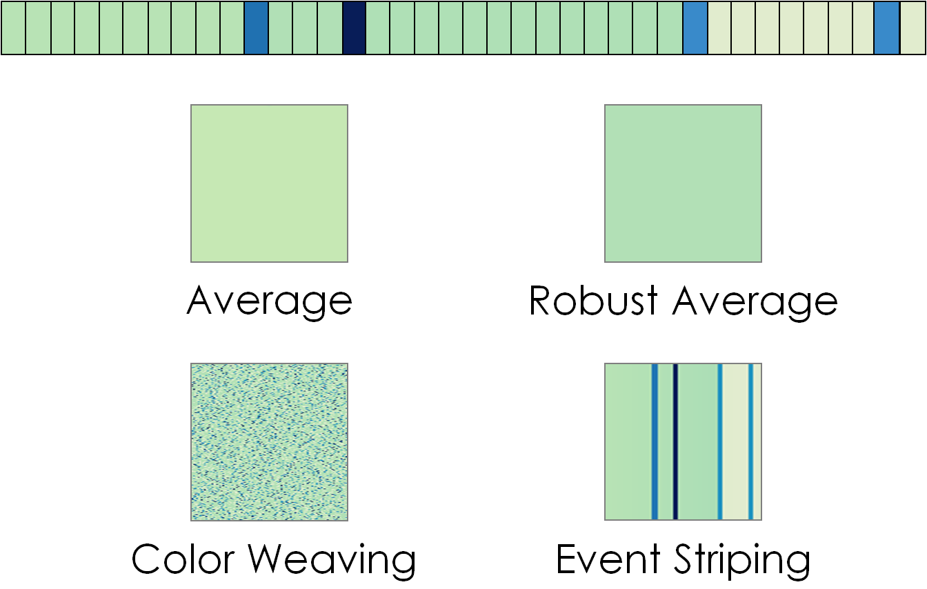
TextDNA supports four visual aggregation types. Here, those aggregate representations are applied to the top sequence of colored elements.
- "Axis" Menu Section: This menu section contains parameter settings for the ordering of elements within sequence rows in the Primary Display and Zoom Window. Manipulating the ordering of elements can highlight specific trends within a dataset by visually clustering like elements.
- "X-Axis" dropdown list: This list defines the setting for the x-axis ordering of elements within a sequence. TextDNA provides four ordering options (Grouped Frequency Ordering, Number of Matches, Position in Reference, and Word Index), all corresponding to their description in the "Color By" dropdown list. For position in reference ordering, the reference sequence can be set using the "Reference" dropdown list immediately below the "X-Axis" dropdown list or by right-clicking on the target sequence and selecting "Set as Position Reference".
- "Normalize block size" radio button: When selected, this box indicates that all elements are represented using the same normalized width. Otherwise, elements are represented using the difference between their start and end values, as specified by the database (see "Data Format" for details).
- "Glyph" Menu Section: This menu section contains the parameters that control spacing and sizing in the Primary Display.
- Block Grouping Width: This parameter defines the minimum width, in pixels, covered by a block. A larger block grouping width implies a greater number of elements will be aggregated into each block and vice versa.
- Glyph Height: This parameter defines how tall each block, an in turn, each sequence will be. By default, this parameter is set to maximize the size of the sequences while keeping all sequence rows visible.
- Vertical Space: This parameter defines how much white space is placed between each sequence. By default, this parameter is set to be approximately half of the glyph height.
- "Update" button: This button applies the settings defined in the Properties menu to the visualization, updating the Primary Display, Histogram, and Zoom Window.
- "Reset" button: This button resets the Properties menu and visualization to the default parameters of the tool.
- "Add Color Ramp" button: This button opens an "Add Color Ramp" dialog box. Colors can be entered by adding a name reference to the "Name" field and a series of color values to the "Values" field. Color values should be entered as red, green, blue. Each component value must be numeric values between 0 and 255 inclusive. Color values should be separated by a semicolon. Custom ramps can be overwritten by adding a new ramp of the same name as an existing ramp. Clicking the "OK" button adds the new color ramp by name to the "Color Scheme" and "Secondary Scheme" dropdown lists to be used as color ramp parameter settings.
- "Cancel" button: This button resets the settings of the "Properties" menu to match those of the current Primary Display.
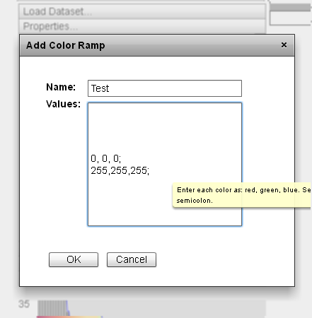 |
The interface to add a custom color ramp requires both a name and a series of color values be entered to define the full ramp. |
Color Scale
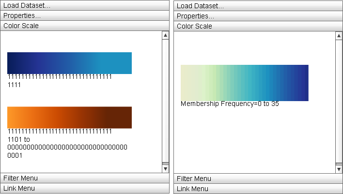 |
The "Color Scale" menu displays the currently active color mappings for the Primary Display. |
The Color Scale menu displays the detailed information about the current color mapping properties of the display: the active ramp is displayed from minimum property value to maximum and the minimum and maximum values are displayed below the ramp. For split color encodings, two ramps are used, one for the first portion of the data (that defined by the "Color Scheme" ramp) and the other for the second (defined by the "Secondary Scheme" ramp).
Filter Menu
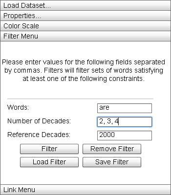 |
The "Filter Menu" allows the user visually filter the data displayed in the Primary Display. |
The Filter Menu allows the user to build conjunctive filters over the dataset. By entering element names in the "Words" field, the number of sequences a set of matching elements can be found in in the "Number of Decades" field, and/or the names of particular sequences to an element must match at least one component element in the "Reference Decades" field, a filter is constructed. Multiple elements can be entered into each field by separating values using a comma. Clicking the "Filter" button will reduce the opacity of any blocks not satisfying at least one of the filter criteria in the Primary Display, and any element not matching the criteria in the Zoom Window.
Clicking on "Remove Filter" will clear the current filter boxes and restore the opactity of all filtered blocks. The "Load Filter" button will open a load file dialog box. Opening a .filter file using this dialog will load the parameters of the filter into the "Filter Menu". The "Save Filter" button will open a save file dialog box to write out the filter parameters to a .filter file. All .filter files are of the format:
words:
<comma-separated list of element names>
frequencies: <comma-separated list of frequencies (matching element set sizes)>
decades: <comma-separated list of sequence names>
Link Menu
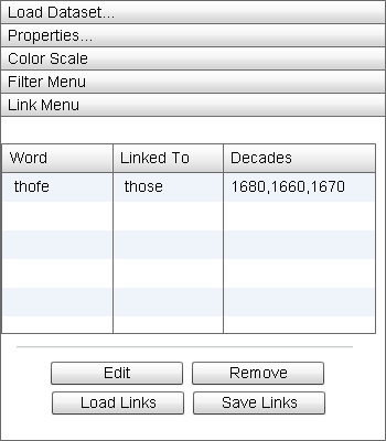 |
The "Link Menu" tracks a series of word pairs of interest across particular decades for later data processing. |
The "Link Menu" can be used to build a .csv file of element pairs for later processing of the dataset. When a block is locked to the Zoom Window (see "Basic Use"), an element can be set as a link element. Linking two elements together opens a link dialog box where the user can select the series of decades over which the first element becomes linked to the second. When the user selects the "OK" button, the new link is then sent to the grid in the Link Menu.
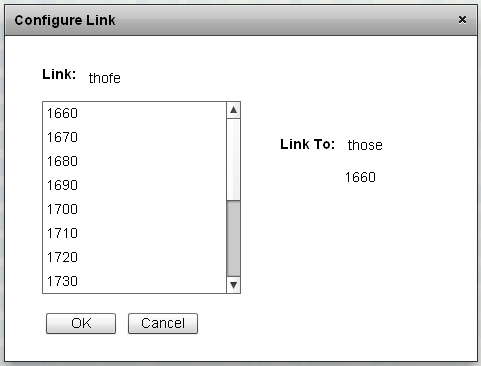 |
The interface to add element links. By selecting a series of sequences on the left, the instances of the left-hand element in those sequences are linked to the right-hand element and sequence in the Link Menu. |
Element in the Link Menu grid can be edited by selecting element and clicking "Edit". This will bring up the original link dialog box, where the user can select a different series of sequences overwhich to link the elements. Selecting a link in the grid and clicking "Remove" deletes the link. Selecting "Load Links" opens a load file dialog box, where the user can navigate to a .csv file of links and load them into the grid. Similarly, the "Save Links" button opens a save file dialog box where the user can save the current grid contents to a .csv file. The format of a link within a .csv file is: <first element name>, <first element sequence>, <second element name>, <second element sequence>. Each link is placed on a unique line. The .csv file can then identify word pairings of interest or be used in the data generation pipeline as a mechanism for refining later datasets.
Project Page | Sequence Surveyor | TextDNA
Adobe AIR must be installed to run Sequence Surveyor and TextDNA.
Email dalbers@cs.wisc.edu for more information.