This is a visual walk-through of the Excel-FU demonstration done in-class by Alper on Wednesday, 2/22. This walk-through uses the data in the nba_players dataset Box folder. We’re using Excel 2016 here, which is available for you to download through Microsoft using your wisc.edu login here: http://office365.com.
Contents
Importing and Excel Tables
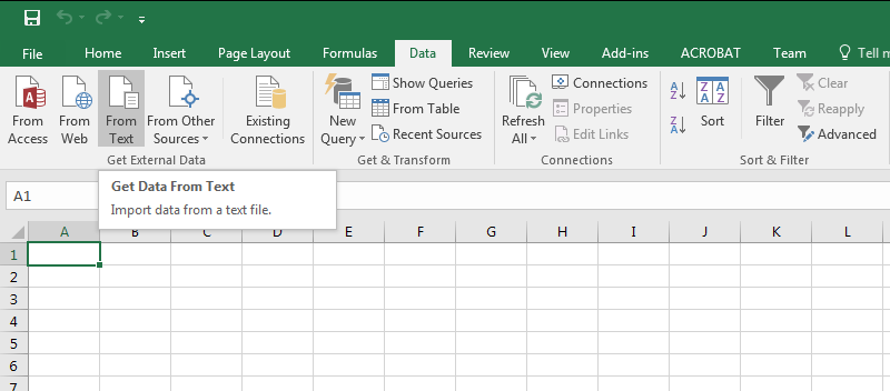
Importing data is always the first step. Let’s import the data through Excel, by going to the Data tab in the Ribbon, then clicking “From Text.”
Select the nba-players.csv file, pass through the first step, select “Comma” as a delimiter, then hit enter to import the data.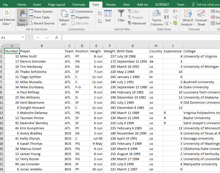
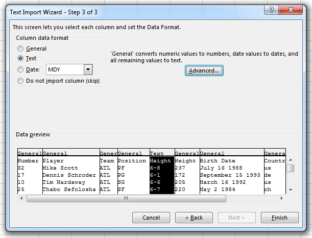
The height column seems to be all goofed up (it’s reporting height as a date), most likely because Excel thought that value was formatted as a date. I can re-run the import process again, by right-clicking the data in the sheet, and selecting the “Edit Text Import…” option. Clicking through the wizard again, pause on the last step. Click on the problem column (Height) and change the column data format to “Text”. This tells Excel not to guess what the column is. Click okay, and see that the data looks okay.
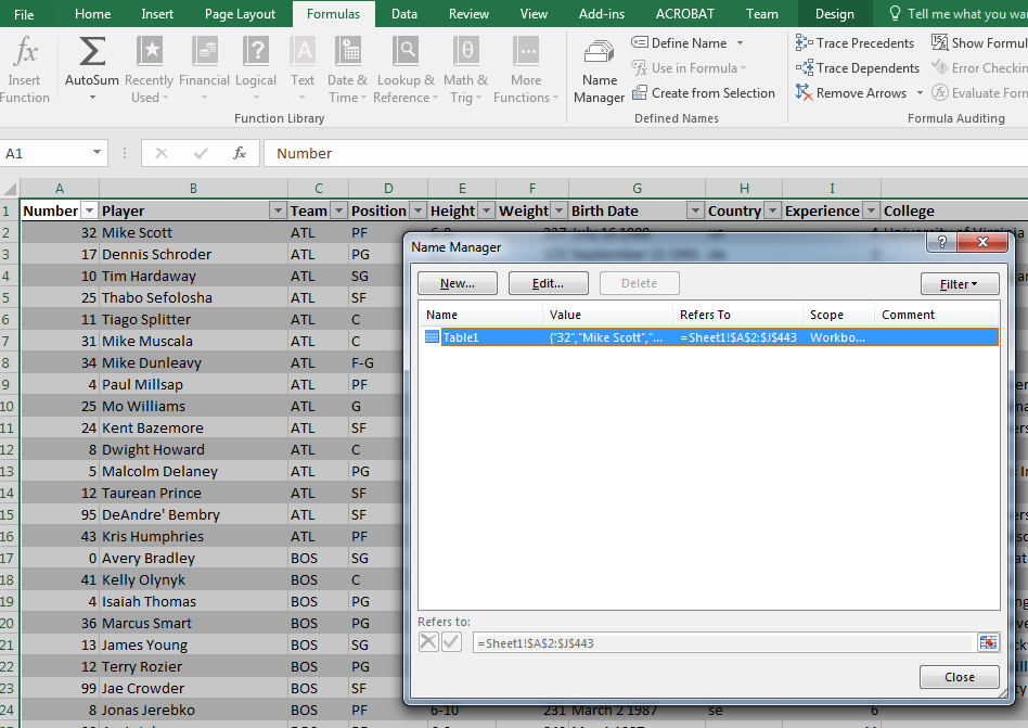
Let’s change this data into an Excel table. This will let us treat the dataset as a named field, and let us make calculations based on columns named by the column names. Select the entire dataset by using Ctrl+Shift+[arrow key] (or Ctrl+A), then under the Home tab in the Ribbon, click the “Format as Table” option, then select a design. This might kill the external CSV import; click OK to continue. You can now use the drop-downs by each column title to filter the items, and make formulae that use the table data (e.g., in another cell, type =SUM(Table1[Number])).
We can name this table so it’s easier to refer to it. Go to the Formula tab in the Ribbon and click “Name Manager” near the middle. We can rename the table to “players”, so now this will be our reference throughout the table.
PivotTables (data aggregation)
We can see some trends over the dataset by using the dimensions and aggregating by the number of players by the values in the dimensions.
Make a new sheet, then create a PivotTable by clicking Insert on the Ribbon, then “PivotTable”. In the data source box, type the name of the table (“players”), then click OK to place it into your new sheet.
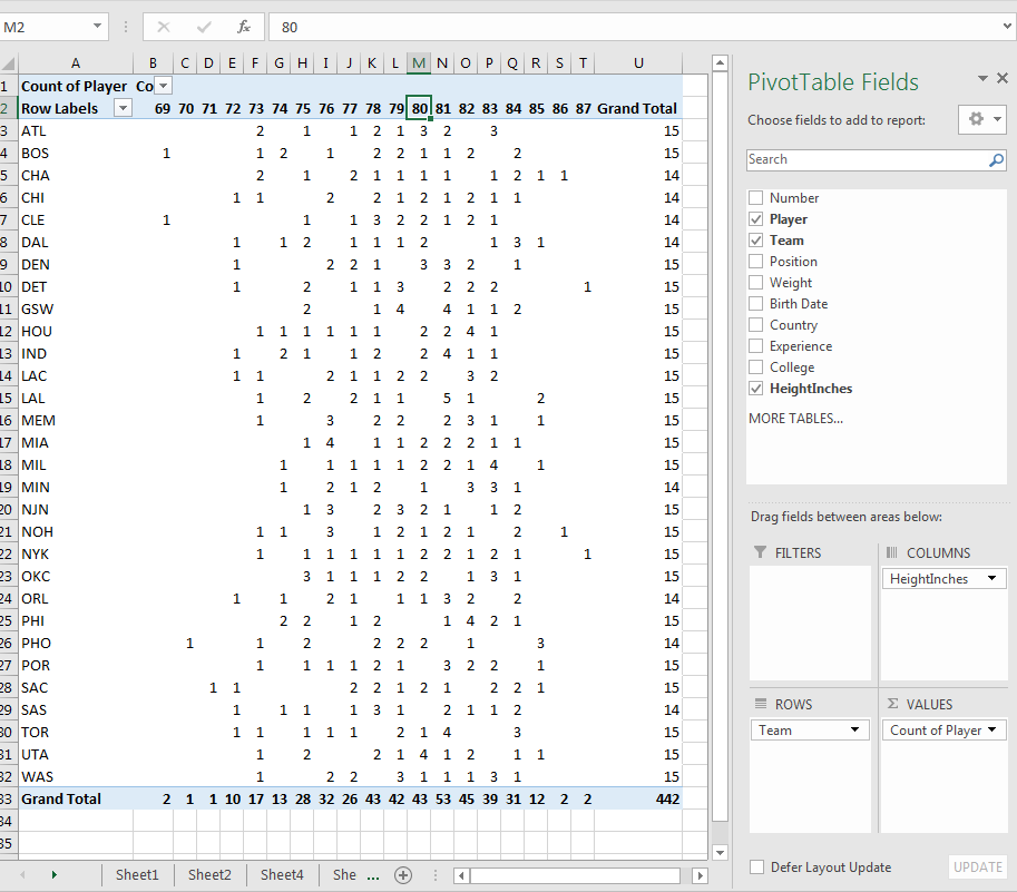
In the PivotTable sidebar, drag “Team” to rows, and “Player” to values. This enumerates all unique teams on the rows, and counts the number of unique players per team. Try out different combinations to see more interesting aggregations: show the experience by team.
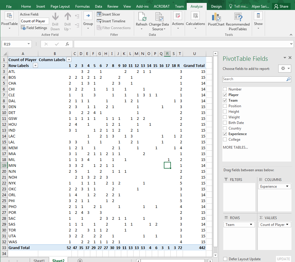
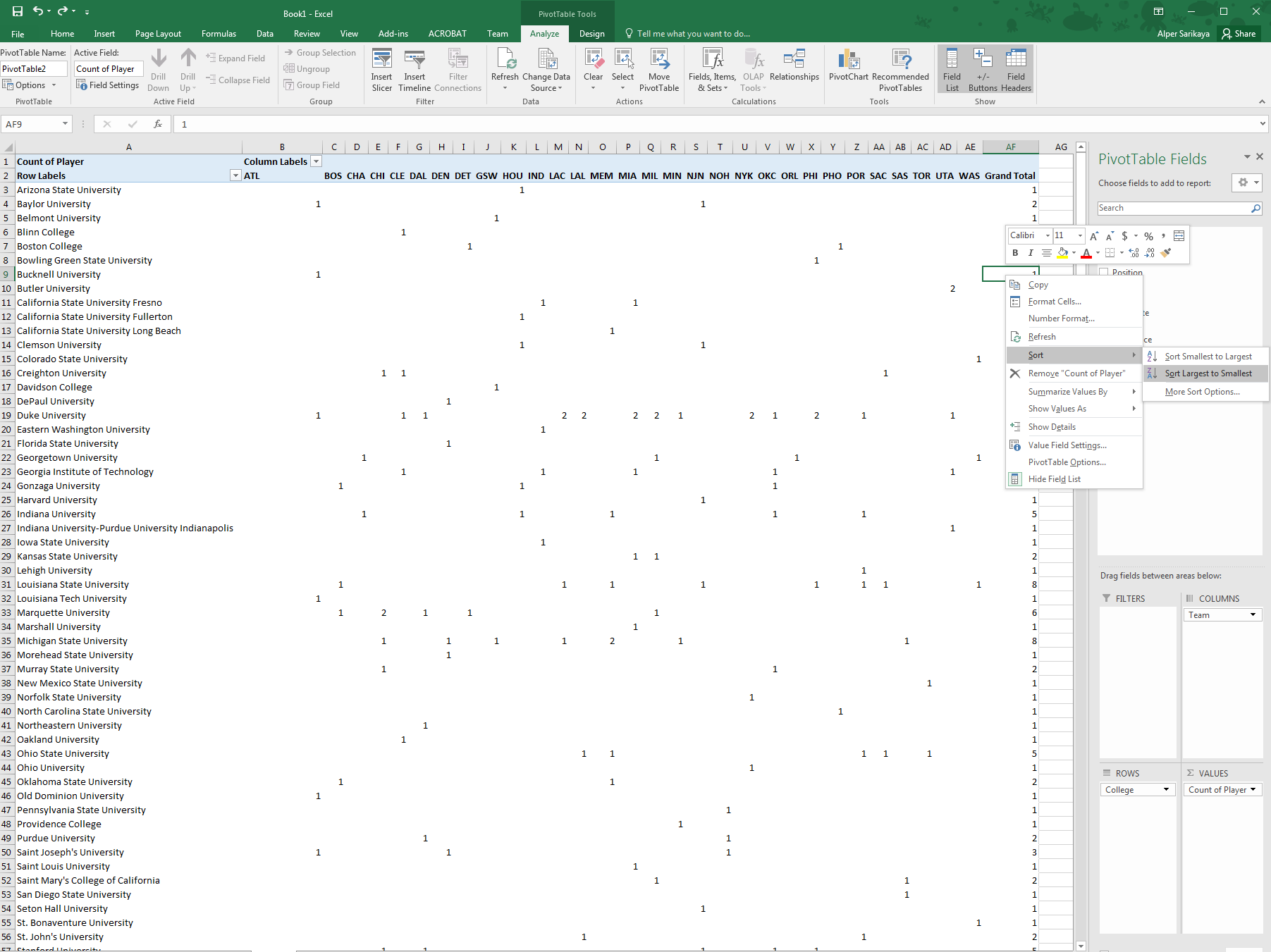
Maybe even the team by the colleges that represent them? If the table gets too big, you can try sorting: right-click one of the totals fields per college, then sort largest to smallest.
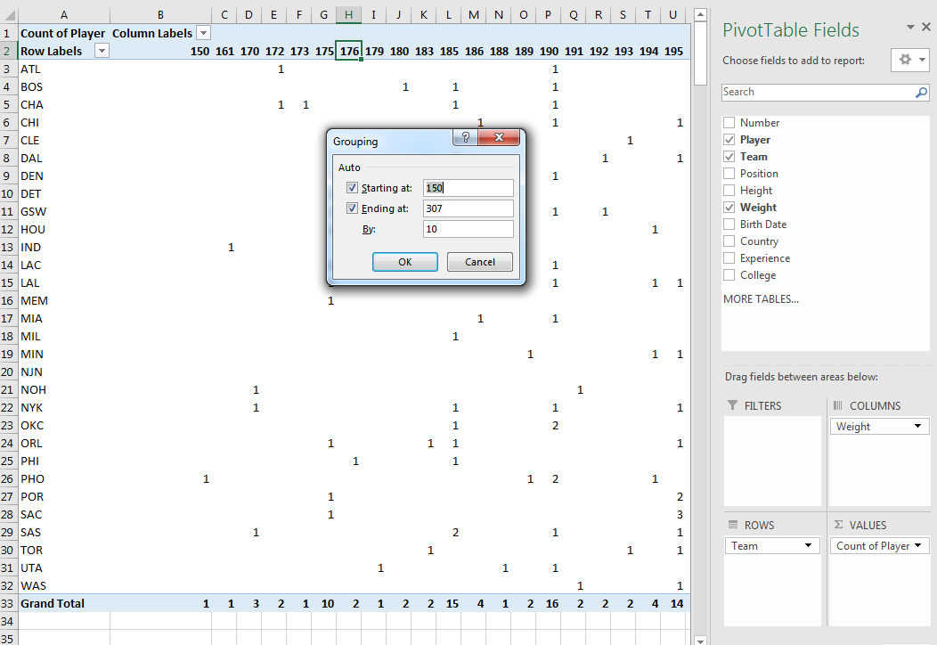
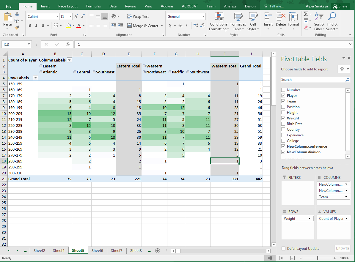
For continuous fields, you can also bin so that each individual value doesn’t get a cell. Right-click on one of the column identifiers that you want to bin, then select “Grouping”. Either accept the default options or insert your desired values.
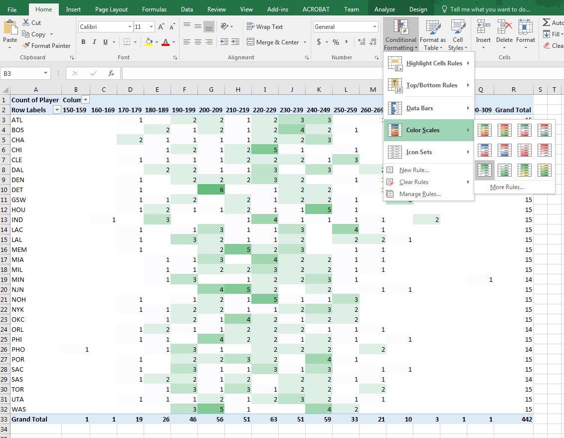
To highlight cells in a heatmap form, select your data range (without including the totals row; this’ll throw off the normalization), then under the Home tab in the Ribbon, select “Conditional Formatting”, then “Color Scales”, then green-to-white ramp. You can modify this rule by clicking “Conditional Formatting” again, clicking “Manage Rules…” at the bottom, then double-clicking your rule to change the color ramp or fix maximum or minimum values.
Using Query Editor
Excel has a handy query editor that can let you do repeatable actions to data to let you clean it. Most importantly, it has a “history” of all the actions that you take to clean, so you can rewind if an issue comes up. The resulting query is able to re-run on the data, even if the source data changes.
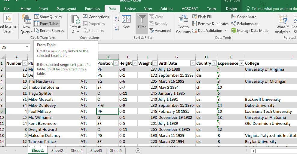
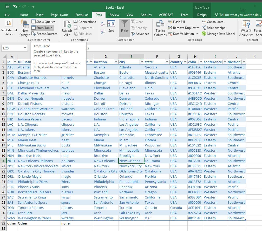
To load your first query, go back to the initial data import (Sheet1), select a cell in the table, then go to the Data tab in the Ribbon, then click “From Table” button within the “Get & Transform” group. This will populate a new query with all data from the table.
The query editor gives a preview of the data. The data is not accessible until you “Save & Load”, which will place the data into a new sheet.
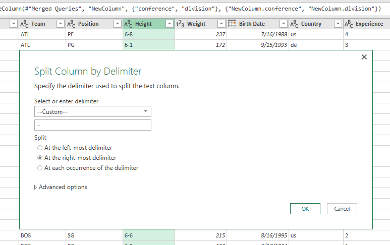
Let’s say that we want to change height into a continuous value: inches. We’ll do this by splitting the column up into the feet and inch components, then making a new derived column. To split the column into its components, click the “Height” column header, then click “Split Column” in the ribbon, then “By Delimiter…”. Select “–Custom–” from the drop-down options, then enter a dash into the text field. Click okay.
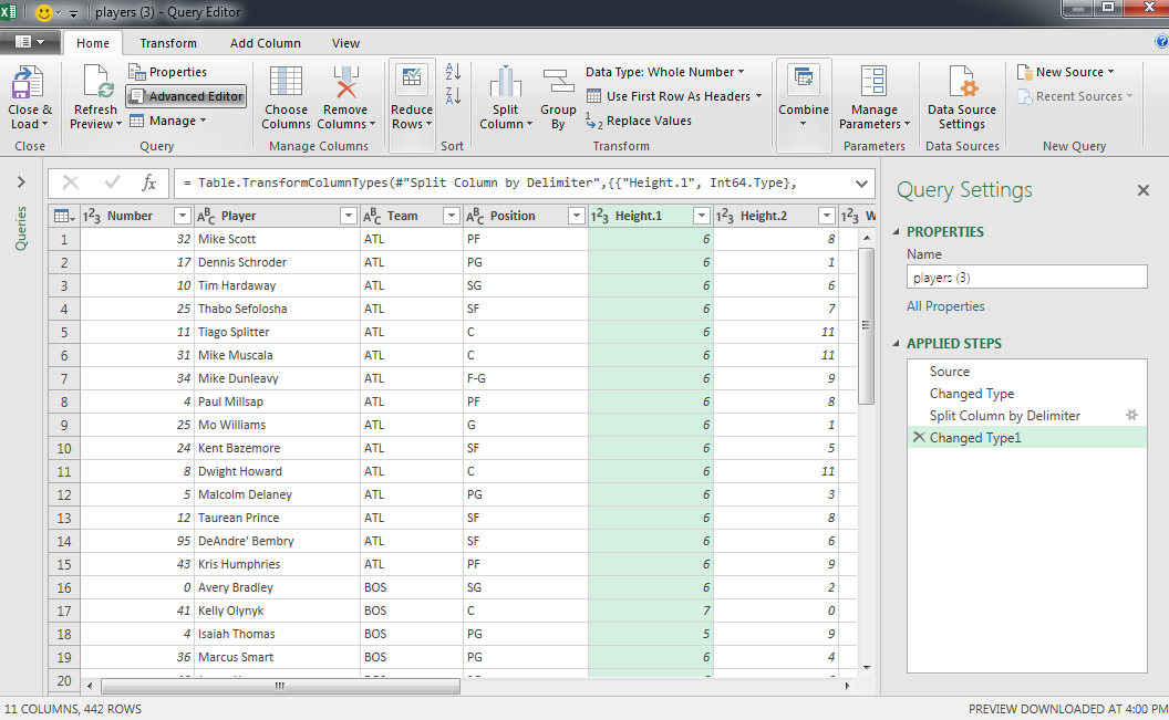
Notice this replaced the original column with Height.1 and Height.2. We’ve also added some steps into the Applied Steps pane, and can reorder or remove these steps if we so choose. All actions we take are recorded in this pane, and we can rewind the data state by clicking on previous actions. Be sure to click on the the last step when adding actions, otherwise you may be making actions out of order.
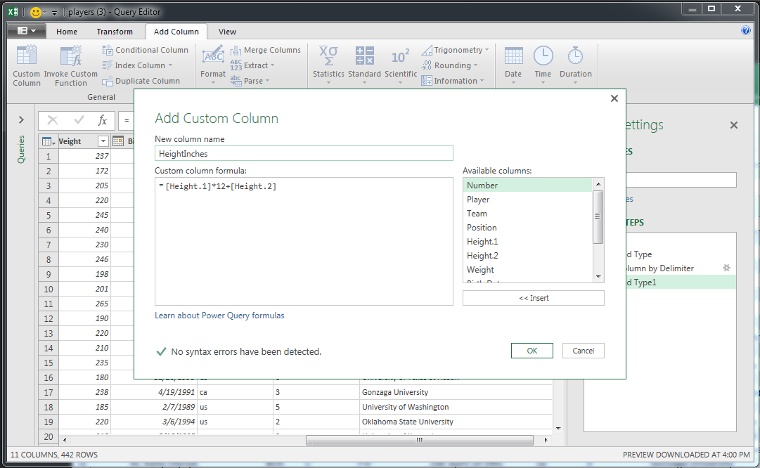
To add a new column, select the Add Column tab in the Ribbon, then click “Custom Column”. We can enter an arbitrary equation here; let’s just put in [Height.1]*12+[Height.2] and rename the column to HeightInches. Hit OK.
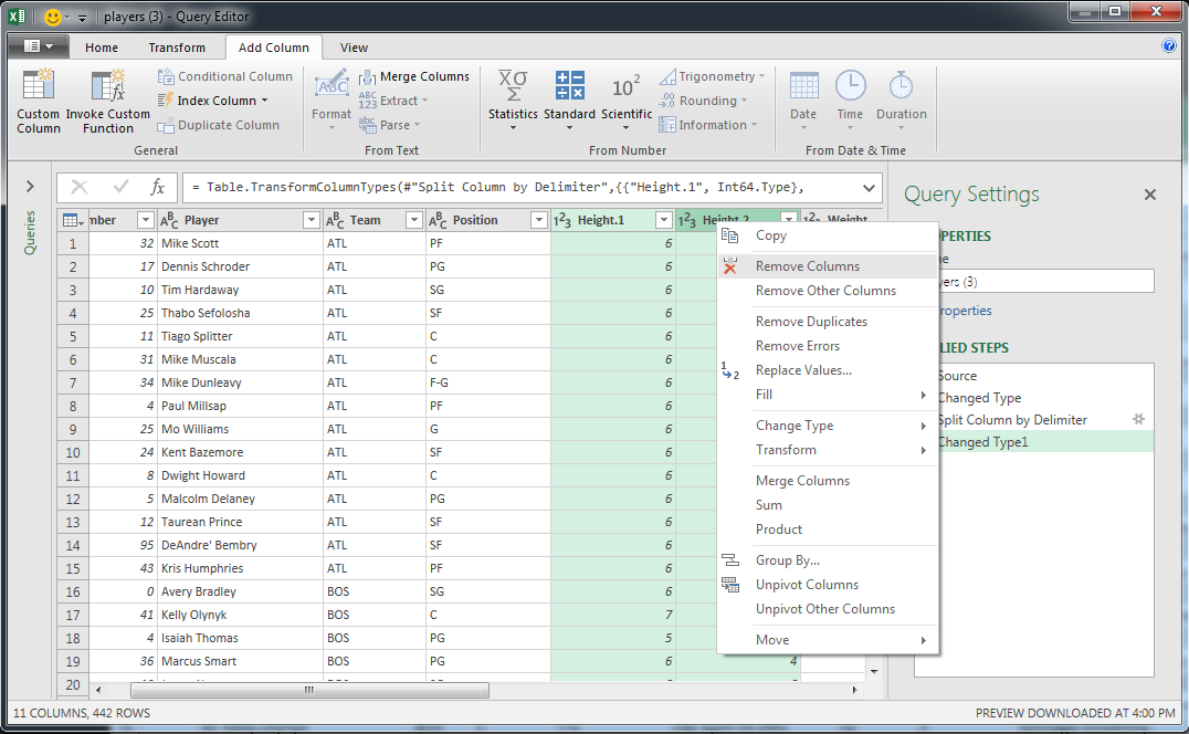
We can remove the two old height columns by selecting them by clicking on their headers, then right-clicking and selecting the “Remove Columns” option. Since this query editor is stateful and has history, we will not have hanging references; HeightInches is still well-defined.
Save the Query by exiting the window and selecting the “Keep” option. A new sheet is populated with your query results. You can again name this table in the Name Manager (call it something like “players_clean”) and can now use the new height field.
Merging Datasets Together
The query editor makes it easy to join multiple datasets together. We will need a field in both datasets that let us join the data together on a common value. In our dataset, the three-letter acronym of the team (e.g., “ATL”) will let us do that. We want some metadata about the team (what conferences and division is each team in) so that we can look at differences of player attributes between conferences and divisions.
Load in your other dataset just like in the first step; we’ll use teams.csv from the Box folder above. Format it as a Table, then open the query editor from table as before.
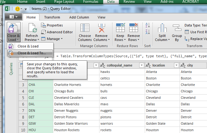
Immediately save and close this query as a connection so that our original query can have access to this data. Do this by clicking “Close & Load” arrow (far-right on the Home tab in the Ribbon), then selecting the “Close & Load To…” option.
In the dialog box, select the “Only Create Connection” radio button, then hit enter. Now, re-enter your original query by finding it in the Workbook Queries sidebar and double-clicking it (if the sidebar is hidden, go to the Data tab in the Ribbon, then click “Show Queries” in the Get & Transform group).
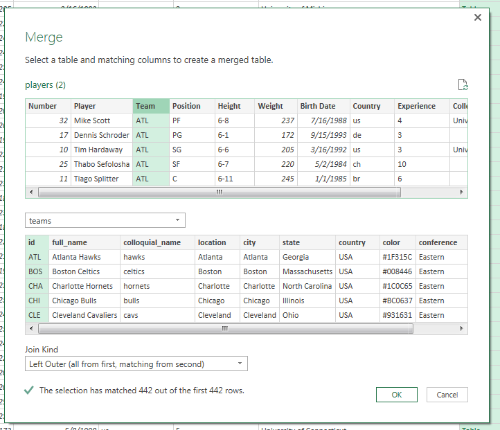
Select “Merge Queries” from the Combine group in the Ribbon. Select the column in the first table to merge on (in our case, “Team”), then select the second table from the dropdown, and the corresponding column in that table. Excel will give a message with a checkmark if the join is successful (the engine finds data for every row). Accept the join by clicking OK.
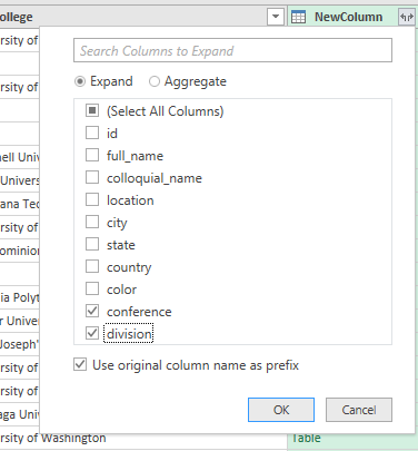
This adds a Table-valued column to the query. To select the fields we want, click the Expand icon next to the column title, and select only “Conference” and “Division”. Click OK.
Save and close the query. The table will update, but you may need to refresh connections to see the new fields in the PivotTable. Click “Refresh All” in the Data tab in the Ribbon. Try creating a hierarchy of conference, then division.
Visualization
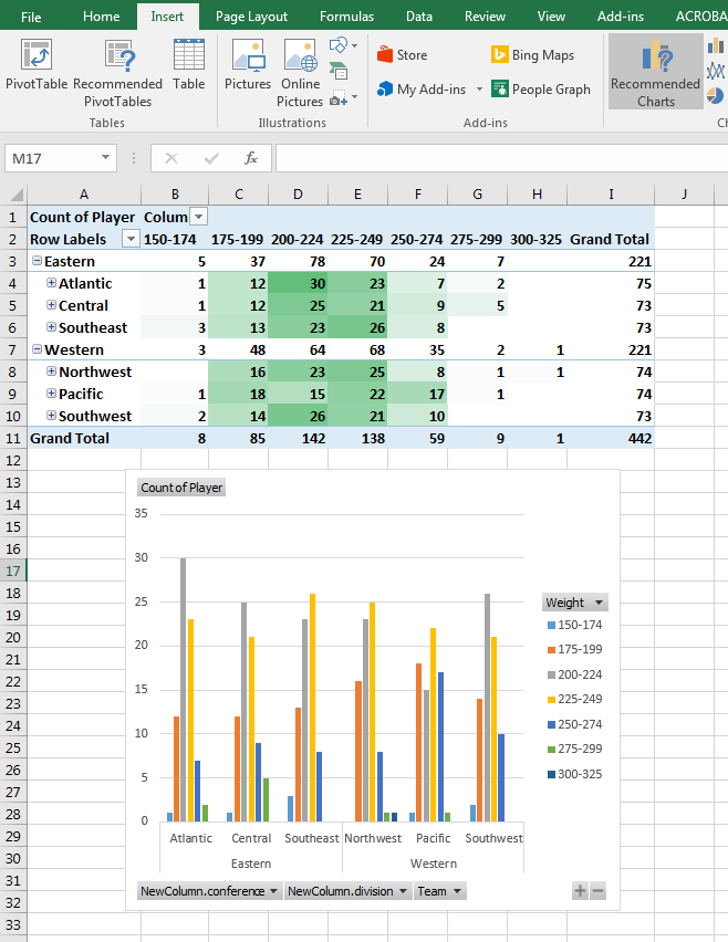
I’d anticipate that you wouldn’t want to use Excel to make a vis, but PivotCharts are actually responsive to your PivotTable! Simply click “Suggested Charts” in the Insert tab in the Ribbon and accept the default “Clustered Column” type by clicking OK. When you change the properties of your PivotTable or expand heirarchies, the graph will follow!
Let us know if you find any other cool tricks with Excel! If you have any comments, please leave them on Piazza or feel free to send me mail.