This is an old version of the page!

Model Selection and Tuning

• Dataset: The data consists of 5044 movies with 27 features, however, 25% is sequestered for final assessment. A stratified sampling of 200 movies per class is held out from the 3756 for testing.

• Classifiers: We develop a classifier to predict movie ratings from IMDB. Classifiers predict a movie’s rating (low, medium, high). A variety of classifiers were constructed such as linear regression(lr), k- neural network(knn), support vector machines(svm), neural network(nn), random forest(rf) and linear discriminant analysis(lda), none with acceptable accuracy.

• Walkthrough:

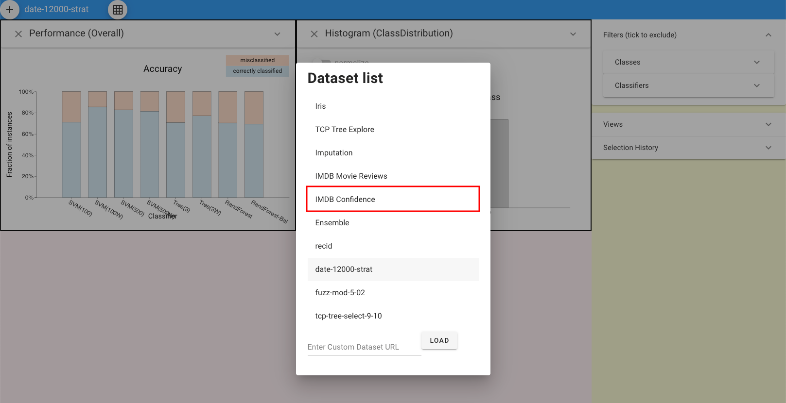
  First, click the button on the top left and load the dataset.

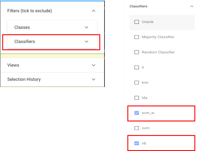
  Since classifier “svm-b” is the classifier after tuning and classifier is the classifier which is not necessary for this use case, let’s first exclude these two classifiers via the selection panel on the right:

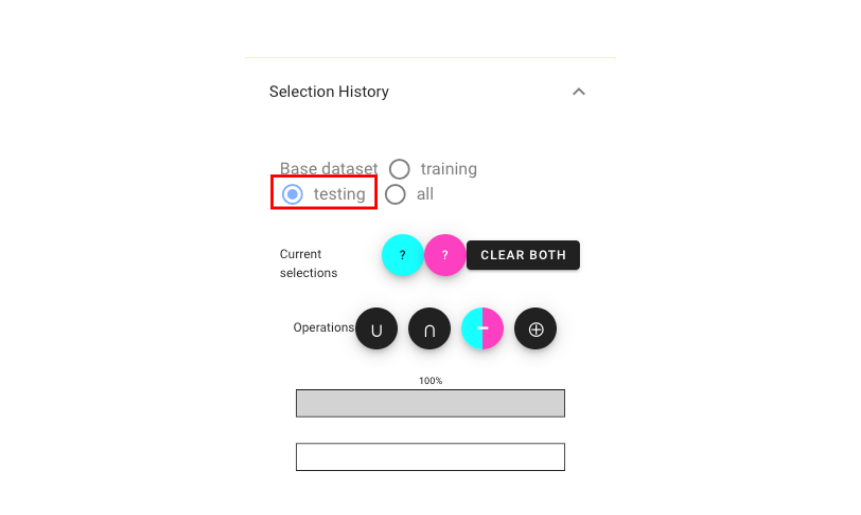
  In addition, we should make sure we are using the “testing” dataset:

  Then, let’s use the Classifier Performance view to see the performance of each classifiers: 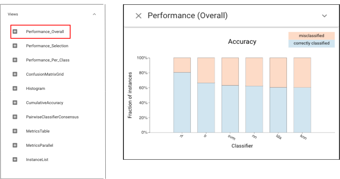This view confirms the poor performance of classifers.

  In order to get more detailed information on those challenging instances, we can apply Cumulative Accuracy view: 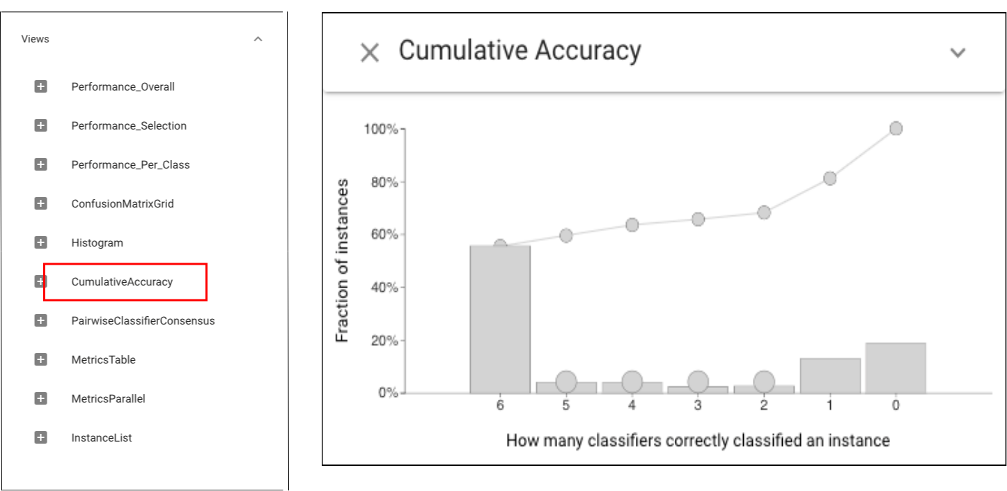The Cumulative Accuracy view shows large numbers of instances that are easy and hard (all or no classifiers are correct).

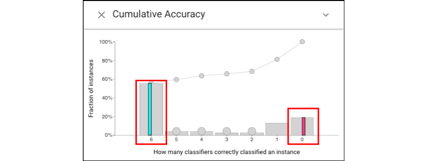
  Let’s select these easy (left click for cyan) and hard subsets (right click for magenta).

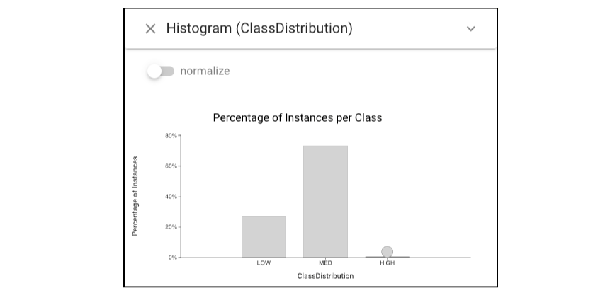
  Open Histogram view of class distribution: 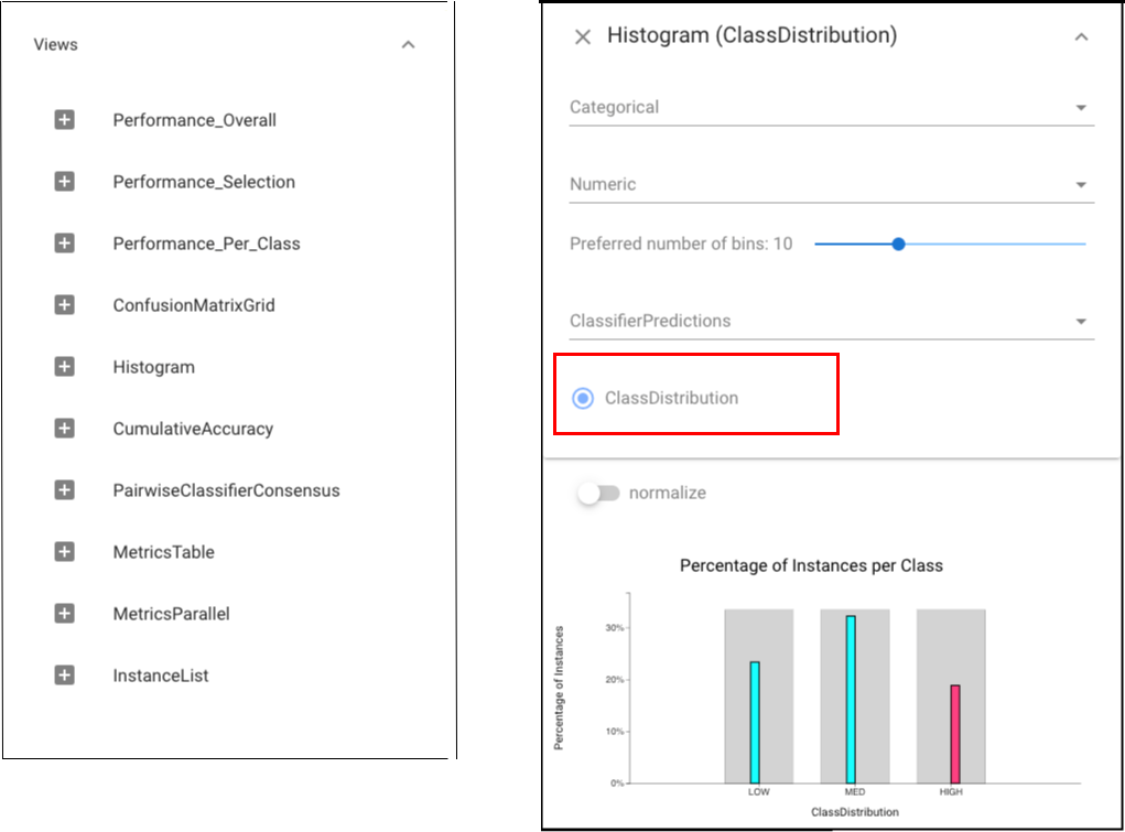In a Histogram view, we can see the hard elements are in the high class, suggesting a skewed training set as shown above.

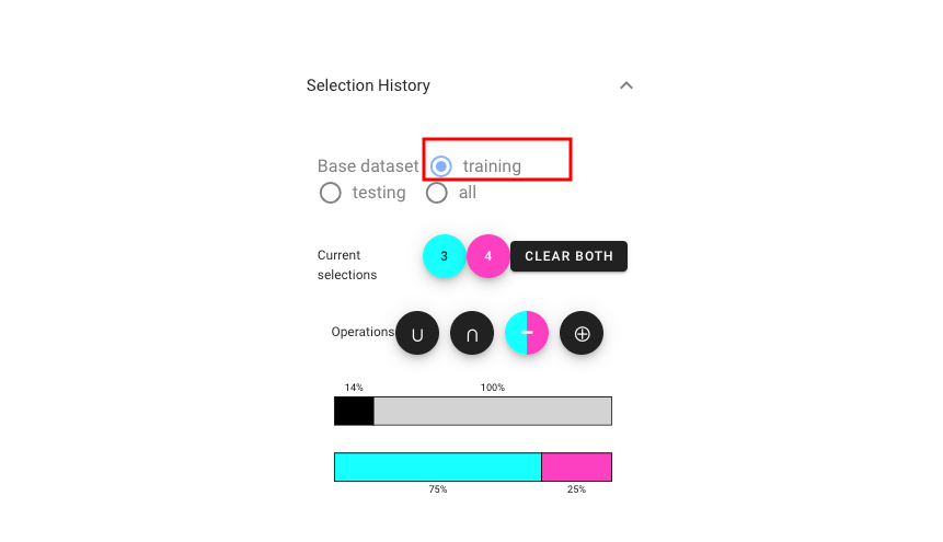
  Now, let’s switch our dataset from “testing” to “training”:

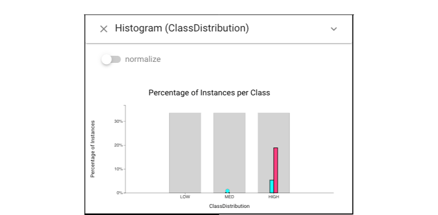
  Back to the Histogram view of class distribution, we can find that this class distribution confirms the skewed nature:

  Therefore, a new classifier called “svm_w” was built that accounts for this skew (now we should include the “svm_w” classifier in the following analysis). Let’s look at the performance of “svm_w” classifier on “testing” dataset.

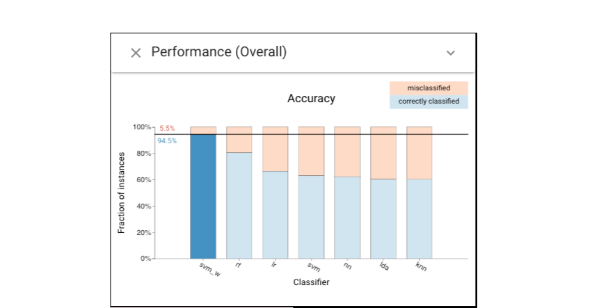
  We can then left-click the misclassified instances of “svm_w” in Classifier Performance view and keep the magenta selection being the same as the previous one. The below Histogram view shows that the new classifier has superior performance, although its errors are still biased.

  In conclusion, while conventional tools can show skew, the example shows how Boxer’s flexible mechanisms allow performance effects to be connected to data issues.